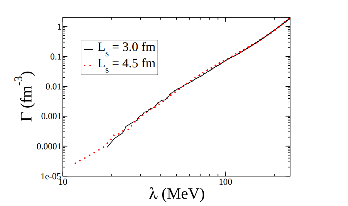
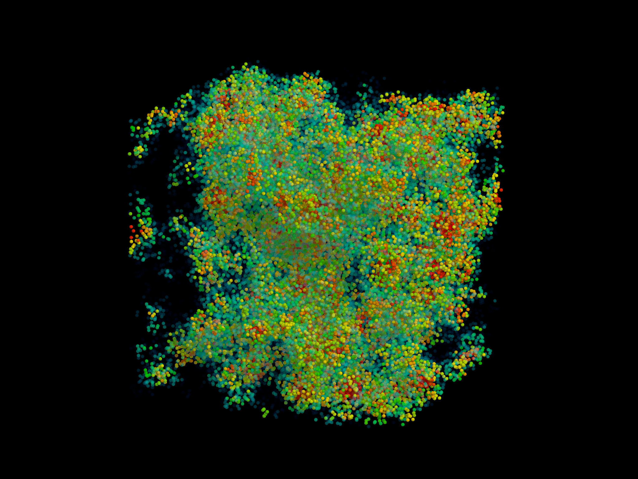
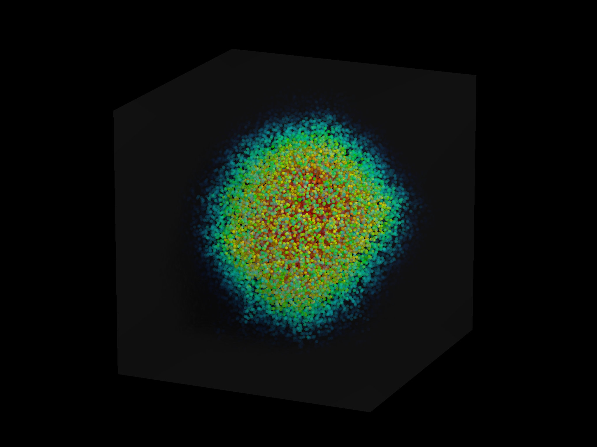
class: center, middle # Lanczos method in High-Performance Computing --- # Agenda - Introduction, linear algebra recap. - The Power method - Krylov subspace - Lanczos method --- # Introduction High performance computing numerical analysis States: Vectors in Hilbert space Measurements: Linear Operators in the Hilbert Space For example in Quantum Chromodynamics $$ S^{QCD}=\int\mathrm{d}^4x\bar{\psi}(x) D \psi(x)+\beta^{-1}\mathrm{tr}F(x)F(x) $$ Fermion states are represented by complex vectors $$ \Psi(x,y,z,t,a,\alpha) $$ a represents color, $\alpha$ spin Observables are Correlation functions: Expectation values of operators --- # Spectrum of D Eigenvectors $$ D\psi=\lambda\psi $$ $\lambda$ is a number Spectral density .center[] Low eigenvalues are important --- # Low eigenmodes of D .center[] .center[] --- # How to differentiate localized-delocalized eigenvectors ? - Eigenvectors are normalized $$ \sum_x \vert \psi(x)\vert ^2 =1 $$ - What happens when we sum the moments of the wave-functions? $$ \sum_x \vert \psi(x)\vert ^4 =? $$ - In the delocalized case $\psi(x)$ does not depend on $x$. $$ \sum_x \vert \psi_0 \vert ^2 = V \psi_0^2 = 1 $$ - Thus for the second moment we get $$ \sum_x \vert \psi_0^4 \vert ^2 = V \psi_0^4 = 1/V $$ --- # The Power method - Given x_0, A - Compute x_1=Ax_0 - x_2=Ax_1 - x_3=Ax_2 - x_4=Ax_3 - Till - x_k=Ax_k-1 approaches the dominant eigenvector --- # Lanczos method Eigenvalues of the Krylov subspace $$ \mathcal{K}(A,v_0)=\lbrace{v_0,Av_0,A^2v_0,A^3v_0,\cdots,A^nv_0\rbrace} $$ Approximate the eigenmodes of $A$ using the Krylov subspace $D$ is sparse $n$ is typically small Storing the subspace is expensive --- # Lanczos method - vector `v_1` be an eigenvector with `| v_1 |- = 1` - beta0 :=0 v0:=0 - for k=1,2,3,... do - w:= A*v_k - alpha_k := (v_k*w) - T_k,k := alpha_k - Diagonalize T^(k) and stop if e_n converges - w := w - beta_(k-1)v_(k-1)-alpha_kv_k - for l=1,2,...,k-2; do - w:=w-v_l(v_l*w) - end for - beta_k=sqrt(w*w) - v_(k+1)=w/beta_k - T_{k,k+1}:=beta_k - T_{k+1,k}:=beta_k - end for --- # Thick Restarted Lanczos - 1: vector v1 be an arbitrary vector with ||v1|| = 1 - 2: kx := 1 - 3: for l = 1, 2, 3, ... do - 4: for k = kx, kx + 1, kx + 2, ..., lm − 1 do - 5: w := Hvk - 6: αk := (vk · w) - 7: Tkk := αk - 8: Diagonalize T(k) and stop if e_n converges - 9: for l = k, k − 1, · · · , 2, 1 do - 10: w := w − vl(vl · w) - 11: end for - 12: βk := |w| - 13: vk+1 := w/βk - 14: Tk,k+1 := βk, Tk+1,k := βk - 15: end for - 16: Construct a new T1(ls+1) matrix and v1, · · · , vls+1 for restart - 17: kx := ls + 1 - 18: end for --- # Implementation details - Question CPU or GPU, which parts are most computationally expensive - Application of the operator - Linear algebra - The following kernels have to be implemented - paxyb : y:=ax+b - scalar product of two vectors - updating the lanczos basis